“`html
Time-Weighted Return: A Performance Measurement Tool
The time-weighted return (TWR), also known as the geometric mean return, is a method of calculating the performance of an investment portfolio that eliminates the distorting effects of cash inflows and outflows. It focuses solely on the investment manager’s skill in selecting and managing investments, making it a more accurate measure of their performance compared to methods like the simple average return.
Understanding the Formula
The core concept of TWR is to break down the investment period into sub-periods defined by external cash flows (deposits or withdrawals). The return for each sub-period is calculated, and then these returns are geometrically linked to arrive at the overall TWR for the entire period. The formula can be expressed as follows:
TWR = [(1 + Return1) * (1 + Return2) * … * (1 + Returnn)] – 1
Where:
- Return1, Return2, …, Returnn are the returns for each sub-period.
Calculating Sub-Period Returns
The most crucial step is calculating the return for each sub-period. This is typically done using the following formula:
Return = (Ending Value – Beginning Value) / Beginning Value
Where:
- Ending Value is the value of the portfolio at the end of the sub-period.
- Beginning Value is the value of the portfolio at the beginning of the sub-period. Critically, this is the value immediately before any cash flow at the start of the sub-period.
A key consideration is that the beginning value of a sub-period is determined *before* any cash inflow or outflow. Conversely, the ending value is determined *after* all investment activity for that period.
Why Time-Weighted Return Matters
The main advantage of TWR is its ability to isolate the investment manager’s performance. Consider a scenario where an investor adds a substantial amount of capital to their portfolio right before a market downturn. A simple return calculation would be heavily influenced by this late-stage inflow, potentially painting a gloomier picture than the manager’s actual stock-picking skills deserve. Conversely, large withdrawals before a period of strong growth would artificially inflate the perceived manager performance.
TWR mitigates these effects. By calculating returns separately for each sub-period, the impact of external cash flows is effectively removed. The geometrically linked returns then reflect the manager’s skill in growing the portfolio with the assets under their control *at that particular time*. This makes TWR a more reliable and objective benchmark for evaluating investment management performance, especially when comparing different managers or assessing performance over time where cash flows are inconsistent.
Example
Suppose a portfolio starts with $100,000. After one year, it grows to $110,000. The investor then adds $50,000, bringing the total to $160,000. In the second year, the portfolio grows to $176,000. To calculate the TWR:
- Period 1 Return: ($110,000 – $100,000) / $100,000 = 10%
- Period 2 Return: ($176,000 – $160,000) / $160,000 = 10%
- TWR = [(1 + 0.10) * (1 + 0.10)] – 1 = 0.21 or 21%
Even though the arithmetic average return is (10% + 10%) / 2 = 10%, the TWR is 21% due to the compounding effect. This demonstrates how TWR accurately reflects the actual growth experienced over the entire investment period, independent of the cash inflow.
“`
 1024×526 weighted average formula calculator excel template from www.educba.com
  910×344 solved puoint problem dollar weighted cheggcom from www.chegg.com
  1200×628 cfa level money weighted return time weighted return soleadea from soleadea.org
  1169×656 time weighted return twr wealthface from wealthface.com
 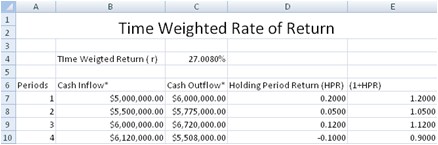 438×145 time weighted rate return from www.spreadsheetml.com
  1050×700 time weighted returns excel template financial analyst from 365financialanalyst.com
  727×235 evaluating investment funds dollar weighted returns from www.verisi.com
  1340×545 calculate time weighted return portfolio performance from www.oldschoolvalue.com